ANOVA: Analysis of Variance

• There are more than two samples/groups, and you want to test for equality of population means among all the groups.

• Example 1: there are four social groups: SC, ST, OBC and Others
  • And you want to test if the average wage of workers belonging to these groups is same.

• Example 2: There are four different Covid vaccines which reduce the severity of impact Covid infection has on patients (say, measured in terms of drop in blood oxygen levels)
  • And you want to test if all the vaccines are equally effective

• Example 3: Three states implemented three different social security programmes
  • And you want to test if all the three interventions were equally effective (say, in terms of average income/consumption of beneficiaries)

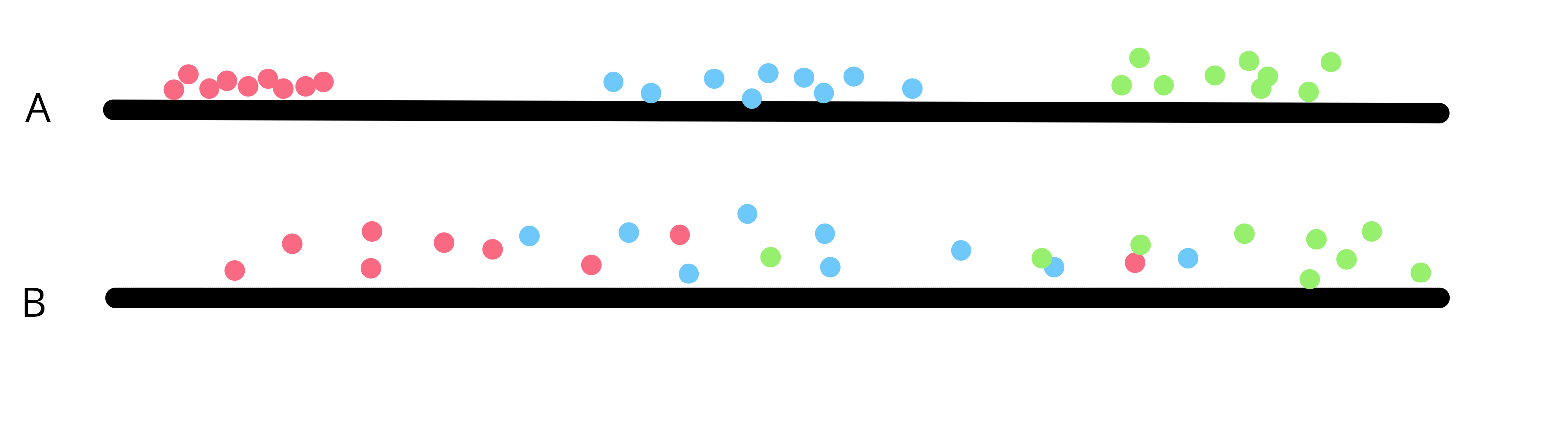
• Greater the variability between sample means of groups and smaller the variability within the sample means of groups, stronger is the evidence that the population means differ
• We create a test statistic that is ratio of estimates of “between group variance” and “within group variance”
• The estimator for within group variance is an unbiased estimator of population variance irrespective of weather H0 is true or not.
• Between group estimator is unbiased only if H0 is true, and in that case, yields a value close to the value of the within group estimate.
• So, we expect the ratio to be close to 1 if H0 is true. It will be higher than 1 if H0 is false.

I

treatments/groups

J

samples in each size (let us assume equal sample size for the sake of simplicity)

\(Y_{i,j}\)

\(j^{th}\) observation of the \(i^{th}\) treatment

• The model:

  \(Y_{i,j}= \mu+\alpha_{i}+\epsilon_{i,j}\)

\(\mu\)

overall mean

\(\alpha_{i}\)

differential effect of the \(i^{th}\) treatment

(no term)

The effect of the treatment is normalised so that: \(\displaystyle\sum_{i=i}^{I}{\alpha_{i}}=0\)

(no term)

\(\epsilon_{i,j}\) are the random errors which are assumed to be independent, normally distributed with zero mean and variance \(\sigma^{2}\)

(no term)

The expected response to \(i^{th}\) treatment: \(E(Y_{i,j})= \mu+\alpha_{i}\)

\(\displaystyle\sum_{i=1}^{I}\sum_{j=1}^{J}{(Y_{ij}-\overline{Y})^{2}}=\sum_{i=1}^{I}\sum_{j=1}^{J}{(Y_{ij}-\overline{Y_{i}})^{2}}+J\sum_{i=1}^{I}{(\overline{Y}_{i}-\overline{Y})^{2}}\)

\(SS_{ToT}=SS_{W}+SS_{B}\)

where \(\displaystyle\overline{Y_{i}}=\frac{1}{J}\sum_{j=1}^{J}{Y_{ij}}\) and \(\displaystyle\overline{Y}=\frac{1}{IJ}\sum_{i=1}^{I}\sum_{j=1}^{J}Y_{ij}\)

\(\displaystyle\sum_{i=1}^{I}\sum_{j=1}^{J}{(Y_{ij}-\overline{Y})^{2}}=\sum_{i=1}^{I}\sum_{j=1}^{J}{[(Y_{ij}-\overline{Y_{i}})+(\overline{Y_{i}}-\overline{Y})]^{2}}\)

\(\displaystyle = \sum_{i=1}^{I}\sum_{j=1}^{J}{(Y_{ij}-\overline{Y_{i}})^{2}}+\sum_{i=1}^{I}\sum_{j=1}^{J}{(Y_{i}-\overline{Y})^{2}}+2\sum_{i=1}^{I}\sum_{j=1}^{J}{(Y_{ij}-\overline{Y_{i}})(\overline{Y_{i}}-\overline{Y})\)

\(\displaystyle = \sum_{i=1}^{I}\sum_{j=1}^{J}{(Y_{ij}-\overline{Y_{i}})^{2}}+\sum_{i=1}^{I}\sum_{j=1}^{J}{(Y_{i}-\overline{Y})^{2}}+2\sum_{i=1}^{I}(\overline{Y_{i}}-\overline{Y})\sum_{j=1}^{J}{(Y_{ij}-\overline{Y_{i}})\)

\(\displaystyle \because \sum_{j=1}^{J}{(Y_{ij}-\overline{Y_{i}})=0\)

\(\displaystyle \therefore \sum_{i=1}^{I}\sum_{j=1}^{J}{(Y_{ij}-\overline{Y})^{2}}=\sum_{i=1}^{I}\sum_{j=1}^{J}{(Y_{ij}-\overline{Y_{i}})^{2}}+\sum_{i=1}^{I}\sum_{j=1}^{J}{(Y_{i}-\overline{Y})^{2}}\)

For \(X_{i}\) where i=1,….,n, be independent random variables with

\(E[X_{i}]=\mu_{i}\), and \(Var(X_{i})=\sigma^{2}\)

It can be shown that:

\(E(X_{i}-\overline{X})^{2}=(\mu_{i}-\overline\mu)^{2}+\frac{n-1}{n}\sigma^{2}\)

where

\(\displaystyle \overline{\mu}=\frac{1}{n}\sum_{i=1}^{n}{\mu_{i}}\)

\(E(U^{2})=[E(U)]^{2}+Var(U)\) for any random variable U with a finite variance

\([E(X_{i}-\overline{X})]^{2}=[E(X_{i})-E(\overline{X}))]^{2}\) \(=(\mu_{i}-\overline{\mu})^{2}\)

\(Var(X_{i}-\overline{X})=Var(X_{i})+Var(\overline{X})-2Cov(X{i},\overline{X})\)

• \(Var(X_{i})=\sigma^{2}\)
• \(Var(\overline{X})=\frac{1}{n}\sigma^{2}\)
• \(Cov(X{i},\overline{X})=\frac{1}{n}\sigma^{2}\)

\(Var(X_{i}-\overline{X})=\frac{n-1}{n}\sigma^{2}\)

• Using \(E(X_{i}-\overline{X})^{2}=(\mu_{i}-\overline\mu)^{2}+\frac{n-1}{n}\sigma^{2}\)
• We can show that \(\displaystyle E(SS_{W})=I(J-1)\sigma^{2}\)

\(\displaystyle E(SS_{W})=\sum_{i=1}^{I}\sum_{j=1}^{J}E(Y_{ij}-\overline{Y_{i}})^{2}\)

\(\because E(Y_{ij})=E(\overline{Y_{i}})=\mu+\alpha_{i}\)

\(\displaystyle E(SS_{W})=\sum_{i=1}^{I}\sum_{j=1}^{J}{\frac{J-1}{J}\sigma^{2}}\)

\(=I(J-1)\sigma^{2}\)

Pooled variance (\(s_{p}^{2}\)) is an unbiased estimator of population variance.

\(\displaystyle s_{p}^{2}=\frac{SS_{W}}{I(J-1)}\) is an unbiased estimator of \(\sigma^{2}\)

\(\displaystyle SS_{W}=\sum_{i=1}^{I}(J-I)s_{i}^{2}\)

\(\displaystyle E(SS_{B})=J\sum_{i=1}^{I}{\alpha_{i}^{2}}+(I-1)\sigma^{2}\)

\(\displaystyle E(SS_{B})=J\sum_{i=1}^{I}{E(\overline{Y_{i}}-\overline{Y})^{2}\)

• Using \(E(X_{i}-\overline{X})^{2}=(\mu_{i}-\overline\mu)^{2}+\frac{n-1}{n}\sigma^{2}\)

\(\displaystyle E(\overline{Y_{i}}-\overline{Y})^{2}=\Big[E(\overline{Y_{i}})-\frac{1}{I}\sum_{i=i}^{I}{E(\overline{Y_{i}})]^{2}]+\frac{I-1}{I}\frac{\sigma^{2}}{J}\)

\(\displaystyle = [\mu+\alpha_{i}-\frac{1}{I}\sum_{i=1}^{I}{(\mu+\alpha_{i})}]^{2}+\frac{I-1}{I}\frac{\sigma^{2}}{J}\)

\(\displaystyle = [\mu+\alpha_{i}-\frac{1}{I}I\mu-\frac{1}{I}\sum_{i=1}^{I}{\alpha_{i}}]^{2}+\frac{I-1}{I}\frac{\sigma^{2}}{J}\)

\(\displaystyle = \alpha_{i}^{2}+\frac{(I-1)\sigma^{2}}{IJ}\), since \(\displaystyle \sum_{i=1}^{I}{\alpha_{i}=0}\) and \(\mu\) s cancel out

\(\displaystyle \therefore E(SS_{B})=J\sum_{i=1}^{I}\Big[\alpha_{i}^{2}+\frac{(I-1)\sigma^{2}}{IJ}\Big]\)

\(\displaystyle =J\sum_{i=1}^{I}{\alpha_{i}^{2}}+(I-1)\sigma^{2}\)

Pooled variance (Sp square) of all samples is an unbiased estimator of population variance.

\(\displaystyle s_{p}^{2}=\frac{SS_{W}}{I(J-1)}\) is an unbiased estimator of \(\sigma^{2}\)

\(\displaystyle SS_{W}=\sum_{i=1}^{I}(J-I)s_{i}^{2}\)

if all the \(\alpha_{i}=0\), then \(\displaystyle \frac{E(SS_{B})}{(I-1)}=\sigma^{2}\)

Thus, this should be the case:

\(\displaystyle \frac{SS_{W}}{I(J-1)} = \frac{SS_{B}}{(I-1)}\)

Since \(\displaystyle E(SS_{B})=J\sum_{i=1}^{I}{\alpha_{i}^{2}}+(I-1)\sigma^{2}\)

If some of the \(\alpha_{i} \ne 0\), \(SS_{B}\) will be inflated

\(H0: \alpha_{1} = \alpha_{2} = \alpha_{3} = ... = 0\) Ha: At least one \(\alpha \ne 0\)

\(F=\frac{SS_{B}/(I-1)}{SS_{W}/[I(J-1)]}\)

follows an F distribution with degrees of freedom I-1 and I(J-1)

If the null hypothesis is true, the F statistic should be close to 1.

If the null hypothesis is false, the F statistic would be inflated.

\(\displaystyle F=\frac{SS_{B}/(I-1)}{SS_{W}/\displaystyle \sum_{i=1}^{I}{(J_{i}-1)}}\) follows an F distribution with degrees of freedom \(\displaystyle \sum_{i=1}^{I}{(J_{i}-1)}\) and I-1