Title slide
(org-show-animate '("Quantitative Methods, Part-II" "Introduction to Statistical Inference" "Vikas Rawal" "" "" ""))
Sampling Distributions
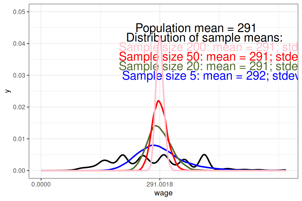
`Sampling Distributions of Sample Mean

Sampling Distributions of Sample Median

Sampling Distributions
- \(Standard.error = \frac{\sigma}{\sqrt{n}}\)
| Variable | Value |
|---|---|
| Standard deviation of population | 130 |
| Standard errors of samples of size | |
| 5 | 58 |
| 20 | 29 |
| 50 | 18 |
| 200 | 9 |
Sampling and Choice of Statistic
| Settlement A | Settlement B | Total | |
|---|---|---|---|
| ACJPuram | 9000 | 1000 | 10000 |
| Sample-I | 180 | 20 | 200 |
| (2%) | (2%) | 2% | |
| Sample-II | 100 | 100 | 200 |
| 1/90 | 1/10 | 2% | |
| Huts | Fancy concrete houses | Total |
Introduction to Hypothesis Testing
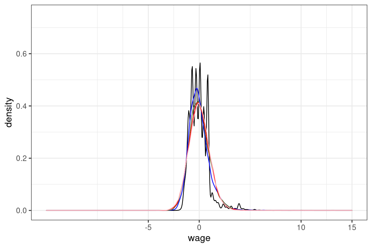
Transforming the Distribution to Standard Normal
\(Z=\frac{x_{i}-\mu}{\sigma}\)

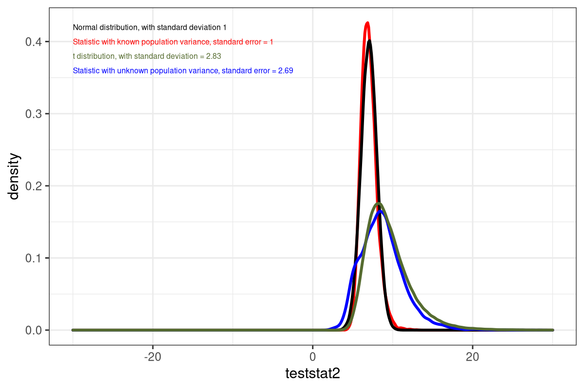
Distribution of sample mean with unknown population variance

Finding an appropriate statistic
Chi-square (\(\chi^{2}\)) distribution
- \(\chi^{2}\) distribution with k degrees of freedom is the distribution of a sum of the squares of k independent standard normal random variables.
if \(X\) is normally distributed with mean \(\mu\) and variance \({\displaystyle \sigma^{2}}\), then:
\(V=(\frac{X - \mu}{\sigma})^{2}=Z^{2}\)
is distributed as a \(\chi^{2}\) distribution with 1 degree of freedom.
- The degrees of freedom in the \(\chi^{2}\) distribution are equal to the number of standard normal random variables being squared and summed. So, the degrees of freedom increase as the sample size increases.
- Properties
- It is a right-skewed distribution.
- Its mean is equal to the degrees of freedom, and its variance is equal to twice the degrees of freedom.
- It is defined only for non-negative values.
Student’s-t distribution
- William Gosset’s 1908 Biometrika paper written with a pseudonym Student.
- t-distribution with df degrees of freedom
If \(Z \sim N(0,1)\) and \(U \sim \chi^{2}_{df}\) are independent then the ratio
\(\frac{Z}{\sqrt{\frac{U}{df}}} \sim t_{df}\)
- Properties:
- It is a bell-shaped distribution that is symmetric around 0.
- Its mean is equal to 0, and its variance is equal to df/(df-2) for df > 2.
- It has heavier tails than the normal distribution.
- For \(df=1\), it is a standard Cauchy distribution
- For \(df \rightarrow \infty, \thickmuskip t_{df} \rightarrow N(0,1)\)
The idea of statistical significance
Key components
- Priors/Assumptions
- Hypotheses
- Test statistic
- p-value
- Inference
Priors/Assumptions
- Scale: discrete/quantitative
- Use of randomisation in generating data
- Population distribution
- Various assumptions may have to be made, usually on the basis of prior information or the sample data, about the underlying population distribution
- For example, about the population variance
- Sample size
The null and the alternative hypotheses
- Null hypothesis (\(H_{0}\))
- Statement that the parameter takes a particular value. Usually to capture no effect or no difference.
- Alternative hypothesis (\(H_{a}\))
- Statement that the parameter does not take this value.
- (no term)
- For example
- For population mean taking a particular value (\(\mu_{0}\))
- H0
- \(\mu = \mu_{0}\)
- Ha
- \(\mu \ne \mu_{0}\)
- For the difference of population means of two groups (say, men and women) being equal to a particular value (\(\mu_{0}\))
- H0
- \(\mu_{a} - \mu_{b} = \mu_{0}\)
- Ha
- \(\mu_{a} - \mu_{b} \ne \mu_{0}\)
- For population mean taking a value higher than a particular value (\(\mu_{0}\))
- H0
- \(\mu > \mu_{0}\)
- Ha
- \(\mu \ngtr \mu_{0}\)
- For population mean taking a particular value (\(\mu_{0}\))
Test statistic
- The difference between the estimate of the test statistic and the parameter value in \(H_{0}\) in terms of number of standard error units.
- For example
For testing that population mean takes a particular value (\(\mu_{0}\))
\(t=\frac{\bar{y}-\mu{0}}{\frac{s}{\sqrt{n}}}\)
For the population means of two groups (say, men and women) being equal
\(t=\frac{\bar{y_{a}}-\bar{y_{b}}}{\frac{s}{\sqrt{n}}}\)
p-value
- We construct the distribution of the test statistic assuming that \(H_{0}\) is true.
- Given the probability distribution, we find out the probability that the test statistic may take the estimated value.
- This is the p-value.
- It gives us the probability that the test statistic equals the observed value or a value even more extreme (in the direction predicted by \(H_{a}\)).
- The smaller the p-value, stronger is the evidence against \(H_{0}\).
- Essentially, we are saying that the data are very unusual if \(H_{0}\) is true.
- The probability at which we reject \(H_{0}\) (usually 0.05 or less) is called the \(\alpha-level\) of the test.
Type I and Type II errors
| Reject \(H_{0}\) | Do not reject \(H_{0}\) | |
|---|---|---|
| \(H_{0}\) is true | Type I Error | |
| \(H_{0}\) is false | Type II Error |
- \(\alpha-level\) is the probability of Type I error.
Chasing the p-values
- \(H_{0}\) may tell a story
- Even if \(H_{0}\) is rejected, the effect may be small