Tests of Significance
1. Introduction
- In statistics, we are often making inferences about the population by looking at a part (sample) of the whole (population).
- This gives rise to uncertainty; whether the inferences made using the sample data about the population are valid or not.
- Tests of significance applied on observed sample data; allows us to measure this uncertainty.
2. Test of Significance
- In a statistical test, we have a null hypothesis and an alternative hypothesis; both referring to the population.
- The null hypothesis is typically a statement of `no difference’ i.e. nothing is happening.
- For example: H0: Mean(male wage) = Mean(female wage)
- In contrast, the alternative hypothesis is a statement that something is happening which is of substantive interest.
- Two-sided: H1: Mean(male wage) ≠ Mean(female wage)
- One-sided: H1: Mean(male wage) > Mean(female wage)
- Using statistical tests we assess whether, based on sample data, we can reject H0 (Null Hypothesis) in favour of H1 (Alternative Hypothesis).
3. Test of Significance
- Note; here we want to decide about population averages using sample averages
- so there is uncertainty involved; risks of making wrong decision
- There are four possibilities involved in a decision:
- Actually H0 is True; Do no reject H0: GREAT! No Error
- Actually H0 is True; Reject H0: Type I Error
- Actually H0 is False; Reject H0: HURRAY! No Error
- Actually H0 is False; Do not reject H0: Type II Error
4. Types of Errors
- Type I error occurs when we reject a true null hypothesis.
- Type II error occurs when we do not reject the null hypothesis when it is not true.
Typically, in a statistical test, we fix the probability of type I error (0.05 or 0.01 by convention) and then minimize the probability of type II error.
- Probability of Type I error is called the level of significance (α)
- When H0 is rejected in favour of H1 at 1% level of significance it means that there is 1% probability that the decision to reject the null hypothesis is wrong.
- OR, the other way of saying is; the statistical test was significant at 1 per cent.
5. Statistical Tests
- There is a wide range of statistical tests that help us reject or not reject our null hypothesis.
- Examples of null hypothesis:
- whether or not population mean is equal to a given constant
- whether or not means of two groups are equal; these groups can be dependent or independent of each other
- whether or not proportions of a variable are equal for two groups
6. Z - test
- Suppose we want to test a hypothesis about mean of a normal population with known variance σ2.
If \(\overline{X}\) is the best estimator of μ0, the following is the best statistic that can be devised.
\(\displaystyle Z = {\frac{\overline{X}-\mu_{0}}{(\sigma/ \sqrt{n})}}\)
- where: \(\overline{X}\) = sample mean, \(\mu_{0}\) = population mean,
- \(\displaystyle \frac{\sigma}{\sqrt{n}}\) = population standard deviation.
7. Z - test
- For example:
- H0: Sample mean is same as the population mean.
- H1: Sample mean is not same as the population mean.
- If the obtained Z value is more than the critical Z value, we reject the null hypothesis.
- Because the population variance is usually never known, in reality, this test is never used.
8. Chi-square distribution
- If Z is a standard normal random variable, the distribution of U = Z2 is called the chi-square distribution with 1 degree of freedom, denoted by χ2.
- It is useful to note that if X ~ N (μ, σ2), then (X - μ)/σ ~ N (0, 1),
- and therefore [(X − μ)/σ]2 ~ χ21 (with 1 degrees of freedom) .
- Chi square distribution with 2 df = (Z1)2 + (Z2)2
- Chi square distribution with 3 df = (Z1)2 + (Z2)2 + (Z3)2 and so on.
- Distribution of χ21 is the distribution of the square of a standard normal variable, and χ2m is the distribution of the sum of squares of m independent standard normal variables.
9. Chi-square distribution
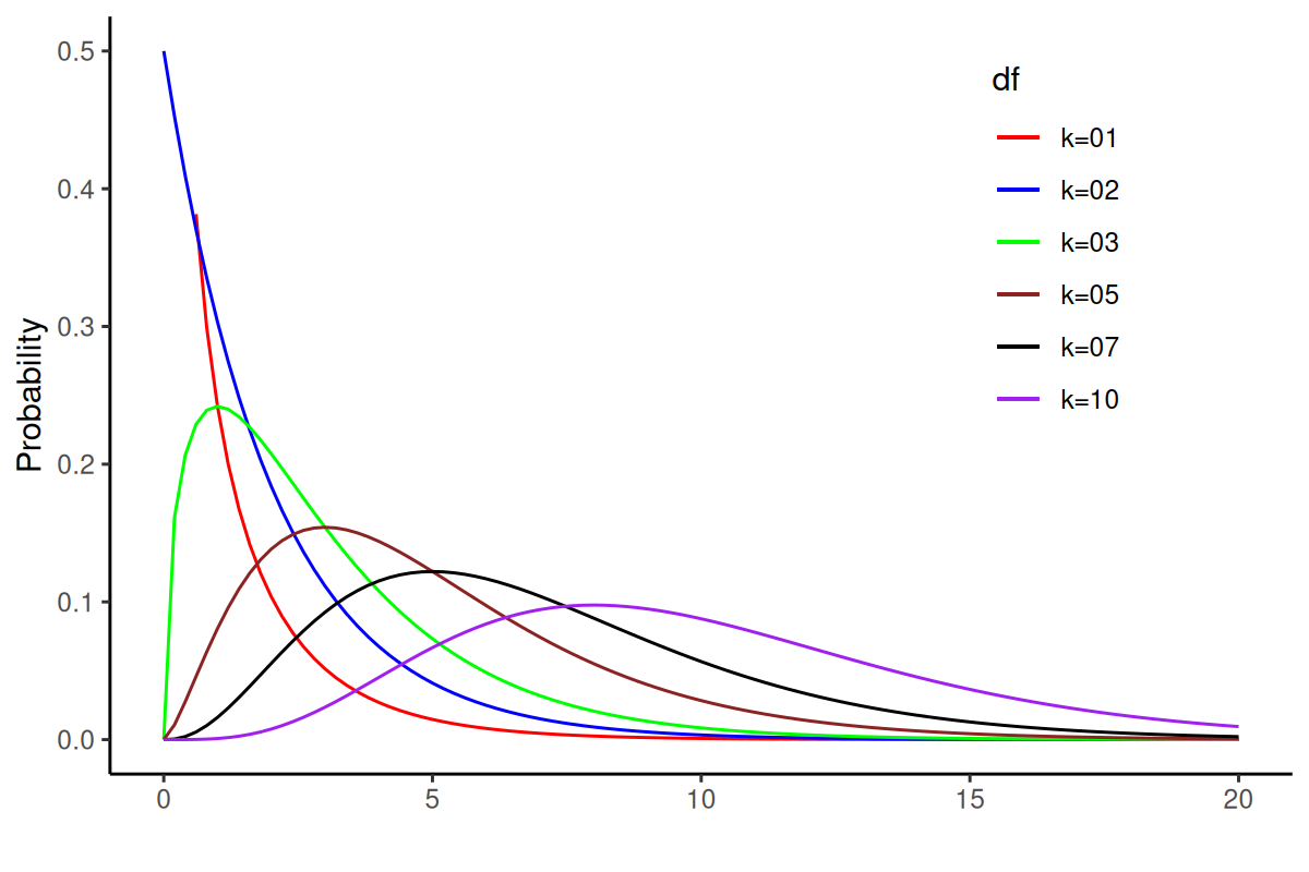
- As degrees of freedom (κ) increases, the distribution looks more and more similar to a normal distribution.
10. Categorical Data: Chi-square Test
- Chi-square tests are hypothesis tests with test statistics that follow a chi-square distribution under the null hypothesis.
- Chi-square test for Independence: To determine if the categorical variables are related/dependent on each other.
- Null Hypothesis: H0: The variables are independent.
- Alternate Hypothesis: H1: The variables are related to each other.
- The chi-square test of independence calculations are based on the observed frequencies, which are the numbers of observations in each category of variable.
- The input data is in the form of a table/matrix that contains the count value/frequency of the variables in the observation – also called a contingency table.
- The test compares the observed frequencies to the frequencies you would expect if the two variables are unrelated.
- When the variables are unrelated, the observed and expected frequencies will be similar.
11. Categorical Data: Chi-square Test
- For example: Households in a locality are supposed to contribute for maintaining the locality garden. All households are randomly divided into three groups and three interventions are tried to assess if any intervention leads to them contributing. First group receives a phone call to explain the importance of having a nice locality garden, second group receives pamphlets with beautiful garden pictures; third is the control group.
- Variable 1: whether or not households contributes
- Variable 2: Type of intervention
- H0: The proportion of households that contribute is same for all interventions (two variables are unrelated).
- H1: The proportion of households that contribute is not same for all interventions (variables are related).
12. Categorical Data: Chi-square Test
Pearson’s chi-square (χ2) is the test statistic for the chi-square test of independence:
\(\displaystyle \chi^{2} = \sum{\frac{(O-E)^2}{E}}\)
- Where
- \(\chi^{2}\) is the chi-square test statistic
- O is the observed frequency in the contingency table
- E is the expected frequency; they are such that the proportions of one variable are the same for all values of the other variable.
- The chi-square test statistic measures how much your observed frequencies differ from the frequencies you would expect if the two variables are unrelated.
13. Categorical Data: Chi-square Test
- The obtained test statistic is compared to a critical value from a chi-square distribution to decide whether it’s big enough to reject the null hypothesis that the two variables are unrelated.
- The critical value in a chi-square critical value table is found using:
- Degrees of freedom (df): (Number of categories in the first variable - 1) * (Number of categories in the second variable - 1)
- Significance level (α)
14. Z - statistic
- Suppose, we want to test a hypothesis about the population mean (μ) of a normally distributed variable (X).
- H0: μ = μ0
- We know, if, \(X ~ N(\mu, \sigma^{2})\),
- then, \(\overline{X} ~ N(\mu, \sigma^{2}/n)\)
Test statistic, if σ known, is
\(Z = {\frac{\overline{X}-\mu_{0}}{(\sigma/ \sqrt{n})}}\)
15. t - statistic
If σ is not known, then the test statistic is given by:
\(t = {\frac {\overline{X}-\mu_{0}}{(s/ \sqrt{n})}}\)
- where: \(\overline{X}\) = sample mean, \(\mu_{0}\) = population mean,
- \(s/\sqrt{n}\) = standard error
- s is the best estimator of σ
- \(s/\sqrt{n}\) = standard error
16. What is the distribution of this statistic?
- By dividing the numerator and denominator by σ and rearranging the result, we get:
- t = \(\frac {(\overline{X}-\mu_{0}) \sqrt{n} / \sigma} {\sqrt{(n-1)s^{2}/(n-1)\sigma^{2}}}\)
- The numerator is the standard normal variable, Z, and the denominator is \((n-1)s^{2}/\sigma_{2}\) = χ2n-1
- t = \(\frac { N(0,1) } {\sqrt{\chi^{2}_{n-1}/(n-1)}}\)
- If Z ~ N(0, 1) and U ~ χ2n and Z and U are independent, then the distribution of \(Z / \sqrt{U/n}\) is called the t distribution with n degrees of freedom.
17. Normal v/s t distribution
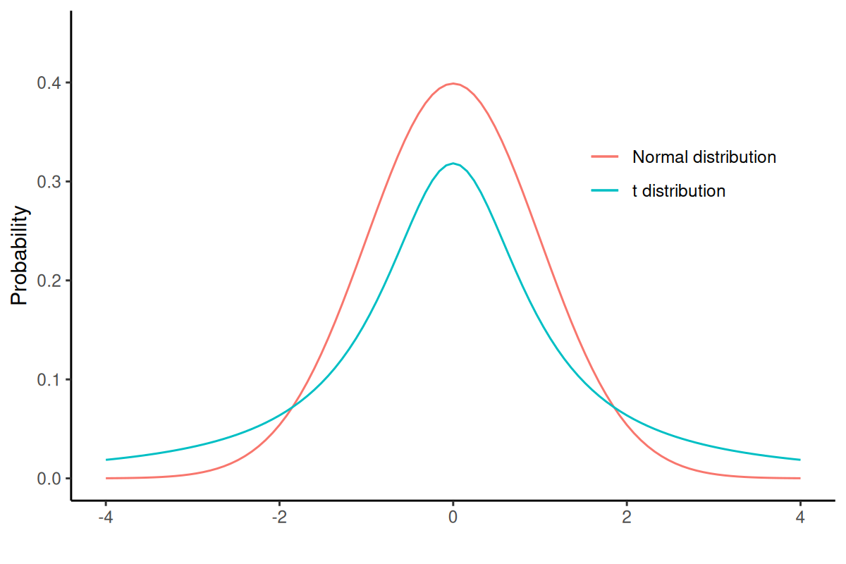
- As the degrees of freedom (total number of observations minus 1) increases, the t-distribution will get closer and closer to matching the normal distribution.
18. t-test: One sample
- One-sample t-test is performed when a sample statistic is compared to a constant given value;
For example: H0: Average wage of women is equal to Rs. 180.
\(t = {\frac {\overline{X}-\mu_{0}}{(s/ \sqrt{n})}}\)
- If tobtained > tcritical, H0 can be rejected.
19. t-test: Two sample
- Two sample un-paired t-test; compares the averages/means of two independent or unrelated groups.
- \(t = \frac{(\overline{X_{1}}-\overline{X_{2}})}{\sqrt{(s^{2}_{1}/n_{1} + s^{2}_{2}/n_{2})}}\)
- \(dof = n_{1} + n_{2} - 2\)
- For example:
- a pharmaceutical study where half of the subjects are assigned to the treatment group and other half are randomly assigned to the control group.
- compare mean wages of men and women workers in a population.
20. t-test: Two sample
- Two sample paired t-test; compares the averages/means and standard deviations of two related groups
- related by being the same group of people, the same item, or being subjected to the same conditions
- t = \(\frac{\sum{(X_{1}-X_{2})}}{s/\sqrt{n}}\)
- \(dof = n - 1\)
- For example:
- before and after effect of a pharmaceutical treatment on the same group of people
- body temperature using two different thermometers on the same group of participants.
21. F-statistic
- Suppose, we want to test a hypothesis that compares the variances of two normal populations:
- H0: σ21 = σ22,
- H1: σ21 > σ22,
- H0 can be tested by drawing a two samples of n1 and n2 sizes and estimating s21 and s22 of the respective variances.
- The appropriate test statistic would be:
- \(s^{2}_{1}/ s^{2}_{2}\) ~ \(F_{n_{1}-1,n_{2}-1}\)
- where s2 are variances of sample 1 and sample 2
- \(s^{2}_{1}/ s^{2}_{2}\) ~ \(F_{n_{1}-1,n_{2}-1}\)
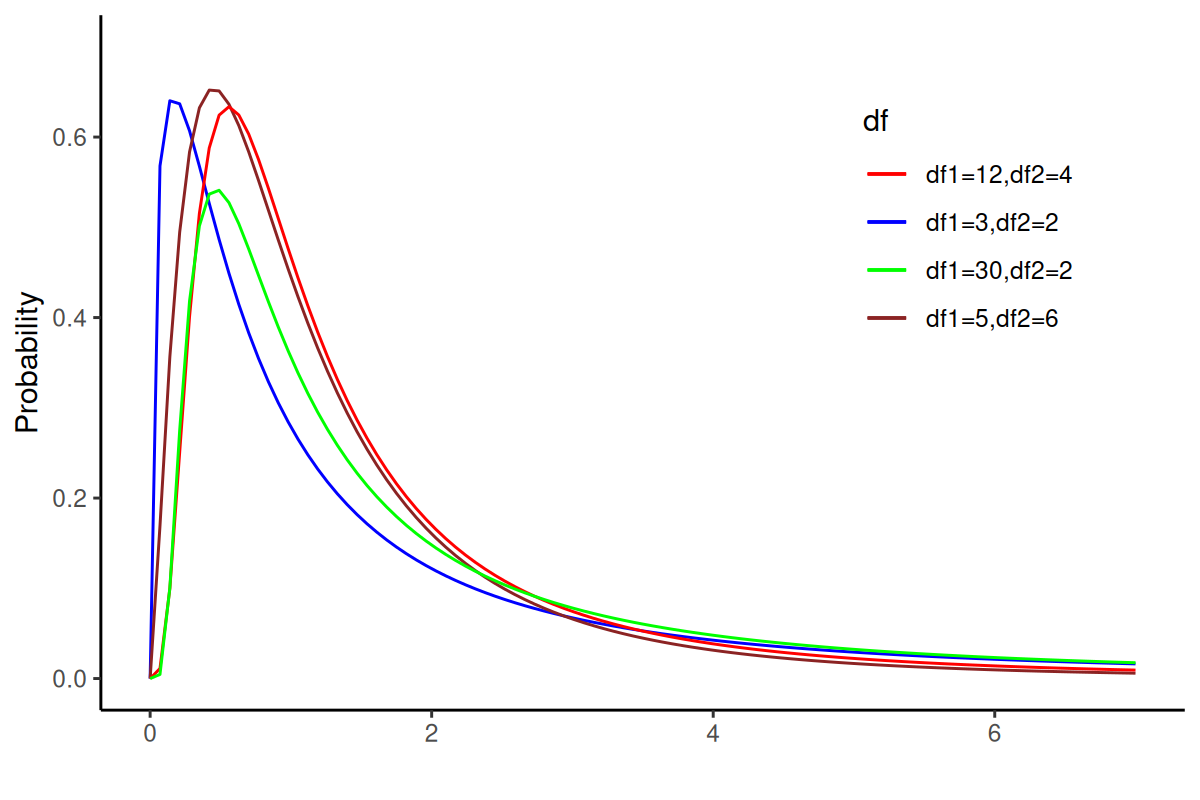
22. F- distribution
- The sampling distribution of the statistic is obtained by dividing the numerator by σ21 and denominator by σ22; if H0 is true, then ratio will be unaffected.
- F = \(\frac{s^{2}_{1}/\sigma^{2}_{1}}{s^{2}_{2}/\sigma^{2}_{2}}\);
- which is equivalent to;
- F = \(\frac{\chi^{2}_{n_{1}-1}/(n_{1}-1)}{\chi^{2}_{n_{2}-1}/(n_{2}-1)}\)
- Let U and V be independent chi-square random variables with m and n degrees of freedom, respectively. The distribution of \(W = \frac {U/m} {V/n}\) is called the F distribution with m and n degrees of freedom.
23. F-distribution